Getting started

DeepPumas.jl contains the neural network infrastructure necessary for the creation of Scientific Machine Learning (SciML) models of longitudinal data, for example, pharmacological modeling, while leveraging the non-linear mixed effects (NLME) functionality of Pumas.jl. There are two ways of enhancing Pumas models with machine learning:

Embedding neural networks directly in a @model (see Embedding Neural Networks in a PumasModel)
Predicting a part of individual variability from baseline covariates via neural networks (see Sequential Covariate Modeling)

In this section, we provide the basic steps for using DeepPumas.jl along with copy-pastable code. For more in-depth details refer to dedicated pages in this or Pumas.jl documentation. The basic steps are as follows:

Get your data ready

Here we generate a synthetic Population of Subjects. The Subject type is generally the workhorse used to represent data in Pumas.jl.

Click to see synthetic data generation

julia

using DeepPumas
using StableRNGs
using CairoMakie
set_theme!(deep_light(), 
)
set_theme!(deep_dark(), 
)

datamodel = @model begin
  @param begin
    tvImax ∈ RealDomain(; lower=0., init=1.1)
    tvIC50 ∈ RealDomain(; lower=0., init=0.8)
    tvKa ∈ RealDomain(; lower=0.)
    tvVc ∈ RealDomain(; lower=0., init=9e-3)
    Ω ∈ PDiagDomain(; init=0.1 * ones(4))
    σ ∈ RealDomain(; lower=0., init=0.2)
  end
  @random η ~ MvNormal(Ω)
  @covariates AGE Weight
  @pre begin
    Ka = tvKa * exp(η[1]) +  0.5 * (AGE/55)^2 
    Imax = tvImax * exp(η[2]) + 1.6*(Weight + AGE)/Weight 
    IC50 = tvIC50 * exp((Weight/75)^2 + η[3])
    Vc   = tvVc * exp(η[4]) * 0.8 * Weight
  end  
  @dynamics begin
    Depot' = - Ka * Depot
    Central' = Ka * Depot - Imax * Central/Vc / (IC50 + Central/Vc)
  end
  @derived begin
    Concentration ~ @. Normal(Central/Vc, σ)
  end
end

pop = map(1:252) do i
  rng = StableRNG(i)
  _subj = Subject(;
    events=DosageRegimen(4.),
    id = i,
    covariates = (; 
      AGE = rand(rng, truncated(Normal(55,10); lower = 15)),
      Weight = rand(rng, truncated(Normal(75,25); lower = 20)),
    )
  )
  sim = simobs(datamodel, _subj, init_params(datamodel); obstimes = 0:0.3:5, rng)
  Subject(sim)
end

trainpop = pop[1:240]
testpop = pop[241:end]

plotgrid(testpop,
  figure=(; resolution=(700,700))
)

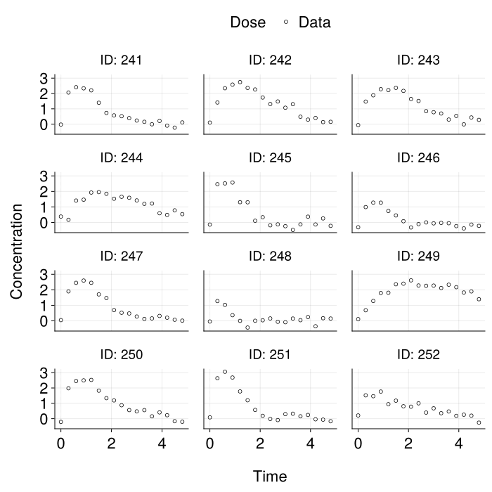
We plot some of the synthetic data that we use for testing trained model performance on.

Define a DeepNLME model

For more details on how to use neural networks in a DeepNLME model see Embedding Neural Networks in a PumasModel.

Click to see DeepNLME model definition

julia

model = @model begin
  @param begin
    NN ∈ MLPDomain(3, 4, 4, (1, identity); reg=L2(1.))
    tvKa ∈ RealDomain(; lower=0.)
    tvVc ∈ RealDomain(; lower=0.)
    Ω ∈ PDiagDomain(4)
    σ ∈ RealDomain(; lower=0.)
  end
  @random begin
    η ~ MvNormal(Ω)
  end
  @pre begin
    Ka = tvKa * exp(η[1])
    Vc = tvVc * exp(η[2])
    iNN = fix(NN, η[3:4])
  end  
  @dynamics begin
    Depot' = - Ka * Depot
    Central' = Ka * Depot - iNN(Central/Vc)[1]
  end
  @derived begin
    Concentration ~ @. Normal(Central/Vc, σ)
  end
end

Fit the defined DeepNLME model to data

For tips and tricks on how to efficiently train DeepNLME models see Performance Tips.

Click to see DeepNLME model fitting

julia

fpm = fit(
  model,
  trainpop,
  init_params(model),
  FOCE(); 
  optim_options = (; iterations=100),
)

true_pred = predict(datamodel, testpop, init_params(datamodel); obstimes=0:0.05:5)

model_pred = predict(model, testpop, coef(fpm); obstimes=0:0.05:5)

plotgrid(model_pred, 
  figure = (; resolution=(700, 700)), 
  pred = (; label = "model pred",
    linestyle=:dash),
  ipred = (; label= "model ipred")
)

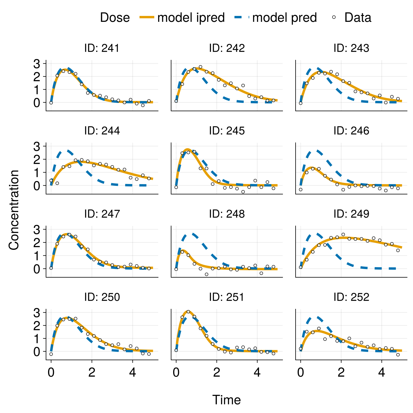
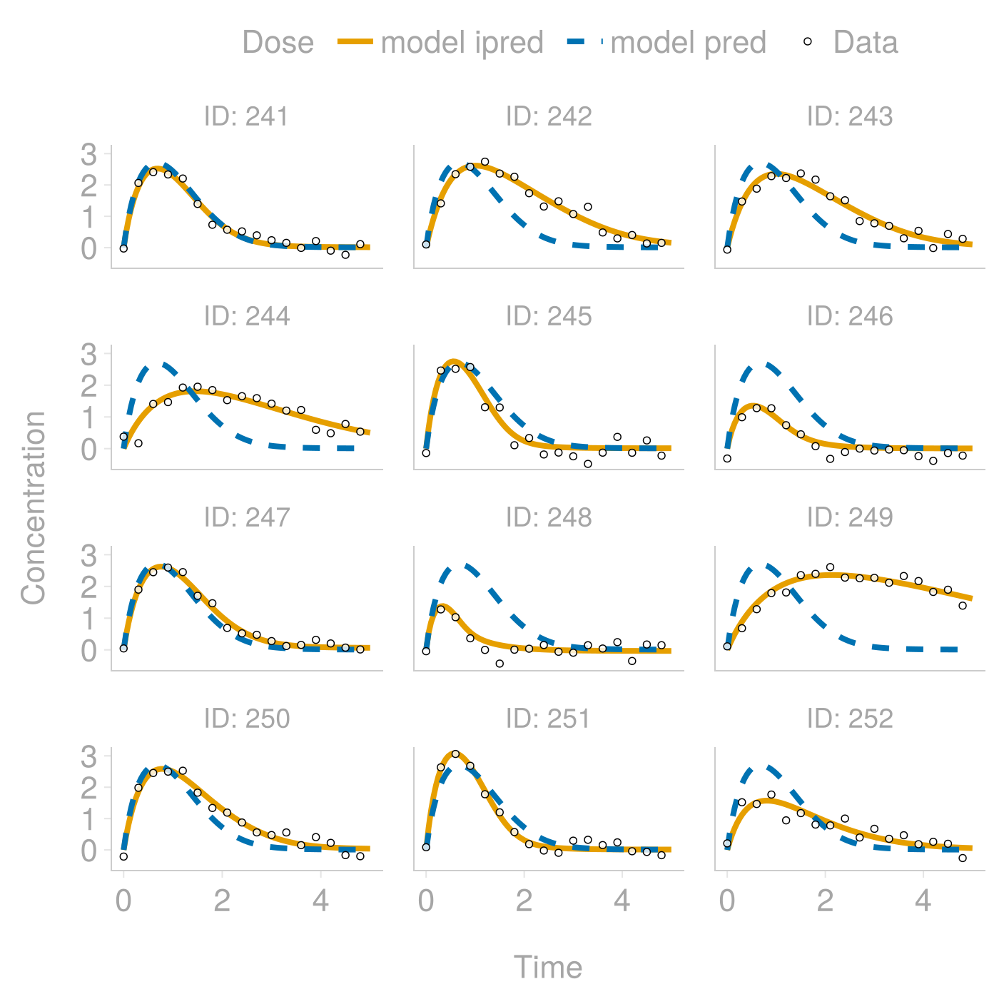
We show the trained model predictions on data that was not used in training. The individual predictions are already accurate, but since we have not yet used the baseline covariates, the population predictions are not tailored to individuals and they are not as good as they could be.

Fit a baseline covariate model to predict some variability in random effects

For more details see Sequential Covariate Modeling.

Click to see covariate modeling

julia

target = preprocess(fpm)
nn = MLPDomain(numinputs(target), 4, 4, (numoutputs(target), identity); reg=L1(0.1; bias=false, output=false))
fitted_nn = hyperopt(nn, target)
covariate_fpm = augment(fpm, fitted_nn)

# The `coef` of an augmented model are the combination of the best parameters of the
# FittedPumasModel and the fitted machine learning model.
covariate_pred = predict(covariate_fpm, testpop; obstimes=0:0.05:5)

plotgrid(
  covariate_pred;
  figure=(;resolution=(700,700)),
  pred = (;
    label="model pred",
    linestyle=:dash
  ),
  ipred = false,
)
plotgrid!(
  true_pred; 
  pred = (; 
    label="best pred", 
    color=(:lightgrey, 0.5)
  ), 
  ipred = false,
)

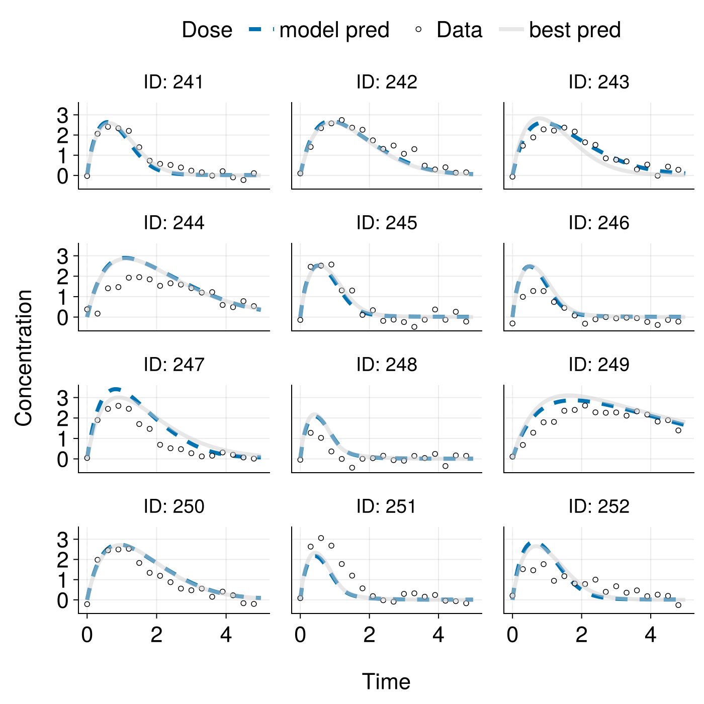
Having fitted a neural network that links covariates to random effects and augmented the model from step 3, we plot the final set of model predictions. This time, we have not only identified a dynamical model flexible enough to individualize descriptions of time courses but also appropriately identified how to individualize predictions based on baseline covariates.

Getting started ​

Getting started