Embedding Neural Networks in a PumasModel

In this section, we describe how to embed a neural network into a PumasModel, how to use it in various @model blocks, and provide practical tips for performance.

Embedding as @param

A standard PumasModel is built using the @model macro, which includes various blocks as described in Defining NLME models in Pumas. The @param macro defines the model's fixed effects and corresponding domains. In DeepPumas, a neural network is an instance of a domain created via MLPDomain (see Neural Network Model Domains). Therefore, we use MLPDomain in the @param block as follows:

@model begin
    @param begin
        ...
        NN ∈ MLPDomain(4, 4, 4, (1, identity); reg=L2(1.0))
        ...
    end
end

Having embedded a neural network NN in our PumasModel, we will now discuss how to use it in the different blocks of a @model.

Using Embedded Neural Networks in @model

Once a neural network is embedded into a PumasModel, it can be used anywhere. Note that neural networks inside a PumasModel are already initialized, unlike those outside of a PumasModel (see Neural Network Model Domains). Therefore, arguments can simply be passed into the neural network, for example, NN(x, y, η). Moreover, the passed vectors are flattened, so NN(x, y, η) == NN(x, y, η[1], η[2], η[3]) if x and y are scalars and η is a 3-dimensional vector. We will showcase the flexibility of neural network usage in DeepPumas.jl via three examples that use different blocks of the @model macro:

1. Linking covariates to patient-specific parameters in the @pre block

2. Discovering terms of a dynamical system in the @dynamics block

3. Linking latent biology to patient measurements in the @derived block

Linking Covariates to Patient-Specific Parameters

One natural way to use neural networks in an NLME context is by combining covariates and random effects into variables for downstream use. This can be done in the @pre block:

@model begin
    @param begin
        ...
        NN ∈ MLPDomain(3, 4, 4, (1, identity); reg=L2(1.0))
        Ω  ∈ RealDomain(;lower=1e-10)
        ...
    end
    @covariates begin
        ...
        AGE
        HEART_RATE_VARIABILITY
        ...
    end
    @random begin
        η ~ Normal(0, Ω)
    end
    @pre begin
        p = NN(η, AGE, HEART_RATE_VARIABILITY)[1]
    end
end

Discovering Terms of a Dynamical System

Another way to use neural networks is to discover individualized dynamical terms in the @dynamics block:

@model begin
    @param begin
        ...
        tv_ka ∈ RealDomain(lower=0.0)
        NN ∈ MLPDomain(2, 4, 4, (1, identity); reg=L2(1.0))
        Ω ∈ PDiagDomain(2)
        ...
    end
    @random begin
        η ~ MvNormal(Ω)
    end
    @pre begin
        ...
        ka = tv_ka * exp(η[1])
        ...
    end
    @dynamics begin
        Depot' = -ka * Depot
        Central' = ka * Depot - NN(Central, η[2])[1]
    end
end

Linking Latent Biology to Patient Measurements

Another way to use neural networks is to link models of latent biology to higher-level observations of patient responses to which the model is fit. This can be done in the @derived block:

@model begin
    @param begin
        ...
        NN ∈ MLPDomain(1, 6, 6, (1, identity); reg=L2(1.0))
        σ_obs ∈ RealDomain(lower=1e-10)
        ...
    end
    ...
    @dynamics begin
        enzyme' = ...
        substrate' = ...
        complex' = ...
        product' = ...
    end
    @derived begin
        patient_response ~ @. Normal(first(NN(Product)), σ_obs)
    end
end

Note that @. converts every functional call/operator into a dot call. Therefore, for operations done on a vector X, @. applies Normal(first(NN(x)), σ_obs) for each x ∈ X.

Fixing Inputs of a Neural Network

Working with complex models and neural networks that mix dynamical variables, covariates, parameters, and random effects inputs may quickly result in messy and difficult-to-read model code. DeepPumas.jl contains the fix function, which fixes some (or all) input dimensions of a neural network – this can be convenient and result in cleaner code.

DeepPumas.fix Function

fix(f, args...)

Return a functor where the first args... arguments of f are flattened, stored, and fixed.

This is conceptually similar to, but faster than, defining x -> f([args..., x]).

source

Using fix, the second example could be written as:

@model begin
    @param begin
        ...
        tv_cl ∈ RealDomain(lower=0.0)
        NN ∈ MLPDomain(2, 4, 4, (1, identity); reg=L2(1.0))
        Ω ∈ PDiagDomain(2)
        ...
    end
    @random begin
        η ~ MvNormal(Ω)
    end
    @pre begin
        ...
        cl = tv_cl * exp(η[1])
        iNN = fix(NN, η[2])
        ...
    end
    @dynamics begin
        Depot' = -cl * Depot
        Central' = cl * Depot - iNN(Central)[1]
    end
end

Performance tips

This subsection contains some practical know-how, performance tips, and theoretical intuitions that should facilitate the efficient use of DeepPumas' functionality.

Choosing a Likelihood Approximation for Fitting

Pumas.jl offers a variety of fitting targets to estimate model parameters, each suited for different scenarios (refer to Estimating Parameters of Pumas Models for a detailed guide). The selection of a fitting target depends on several factors: the volume of available data, the required precision of the model, the available time and computational resources, and the complexity of the model. Given the diverse scenarios that might arise, we will discuss each factor individually–highlighting important considerations–and leave the user to weigh these trade-offs according to their specific context. Roughly speaking, we can order the most relevant likelihood approximations in terms of both the generalization performance of the fitted models and the computational time needed to fit. In descending order:

1. LaplaceI - a Laplace approximation of the marginalization of the random effects from the likelihood of the fixed effects.

2. FOCE - a first-order conditional approximation of the marginalization of the random effects from the likelihood of the fixed effects. This can be viewed as a simplification of the Laplace approximation.

3. FO - a first-order approximation of the marginalization of the random effects from the likelihood of the fixed effects. This can be viewed as a simplification of the FOCE approximation.

4. JointMAP - the joint maximum a-posteriori of the fixed and random effects. This avoids marginalization altogether.

5. NaivePooled - the likelihood of the fixed effects conditional on the random effects being set to the mode of their prior distribution. This is usually too simplistic for good generalization performance on longitudinal data but is useful for single time-course data or as a first step in a sequential fitting approach.

The computational time for fitting a model scales with both the model complexity and the size of the data used for training. Methods like LaplaceI may be prohibitively expensive when fitting a complex model on large datasets. Then, simpler methods like JointMAP may be more appropriate–especially since we expect the gap in generalization performance to shrink as the training data set increases.

You might also consider using multiple likelihood approximations sequentially–for example, you can find a rough fit for a model by using JointMAP and then refine it further via FOCE (or some other combination of fitting targets).

Input Scaling

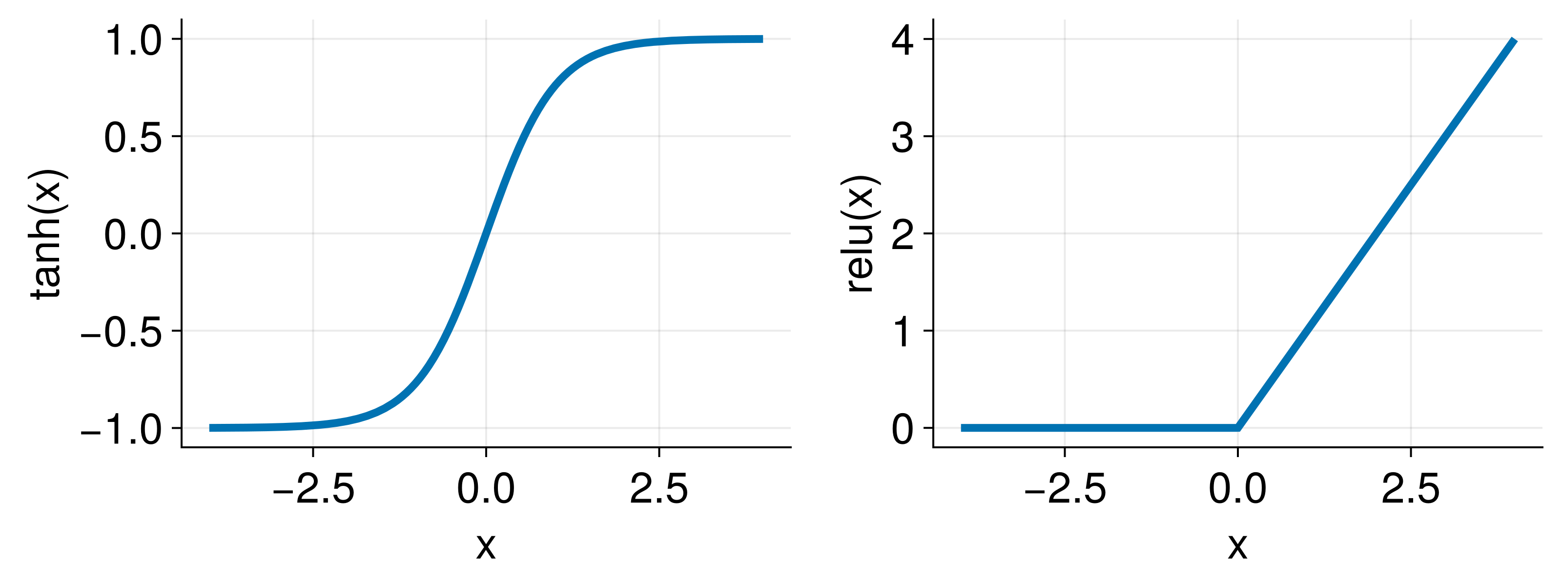
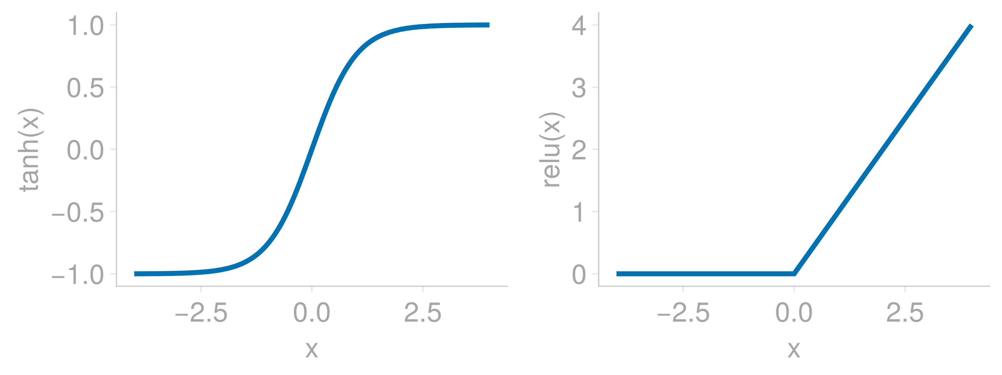
Scaling the inputs of neural networks is a standard practice in machine learning that helps to avoid vanishing gradients due to the saturation of activation functions. As an example, consider two popular activation functions tanh and relu whose functional shape is shown below

Note how the tanh output saturates at large positive or negative $x$ values, and relu output is zero when $x<0$ by definition. In these regions of the input space, the gradients with respect to neural network parameters will be either very close to or exactly zero. This impedes model training and should be avoided. One of the easiest ways to avoid this saturation of activation functions is via scaling of its inputs x, for example

• If you know the order of magnitude of x is consistently in the range of ${10}^6$ you can multiply it by ${10}^{-6}$ to bring it into the favorable region of a tanh activation function

• If you know the relevant statistical properties of the input variable, you can convert it to z-scores via z_i = (x_i - mean(x))/std(x).

Output Scaling

Similarly to the scale of the inputs of a neural network, the scale of its outputs is also a practically relevant consideration. Two factors to consider are the domain and the order of magnitude of the neural network outputs. We discuss output layer domains in Choosing Activation Functions and here focus on its order of magnitude.

Even though a neural network may have the correct output domain (e.g. strictly positive via softplus), if the order of magnitude of its output is significantly different from what it should be in the context of a specific model, it may cause issues in fitting. For example, if a neural network is used in the @dynamics to model derivatives and its initial outputs are on the order of ${10}^0$, whereas the rest of the system operates on the order of ${10}^3$, this can lead to small gradients that impede training. Another example is the use of a neural network in the @derived block. There may be a mismatch between the order of magnitude of the output of the neural network and the data to which it is being fit. In these examples, scaling the outputs of a neural network by the scale of the system or the maximal value of the data may facilitate model fitting. Note that while hard-coding such scaling into the model definition is often convenient, one could also do the scaling as a part of data preprocessing.

Regularization Customization

This section ties together and elaborates on practical problems that can be addressed by appropriately customizing a neural network's regularization.

Addressing Input/Output Scaling via Regularization

As mentioned in Input Scaling and Output Scaling there are situations in which the scale of the state variables in a dynamical system may lead to small gradients that cause problems with fitting. One solution for this problem that involves user-defined scaling of inputs/outputs is described above. Unfortunately, this may not always be a possible solution if a state variable has a significant dynamical range and/or the scales are not consistent between individuals. In such cases, even though it is not an easy task, we can leave the learning of the input/output scales to the neural network by turning off input/output regularization. If we use an L1 regularization, the code would be

NN = MLPDomain(5, 10, 10, 5; reg=L1(1.0, output=false, input=false))

In addition to customizing the regularization, we can also adjust the activation functions, see Choosing Activation Functions below.

Intuition Behind L1 and L2 Penalties and Ties to Probability Distributions

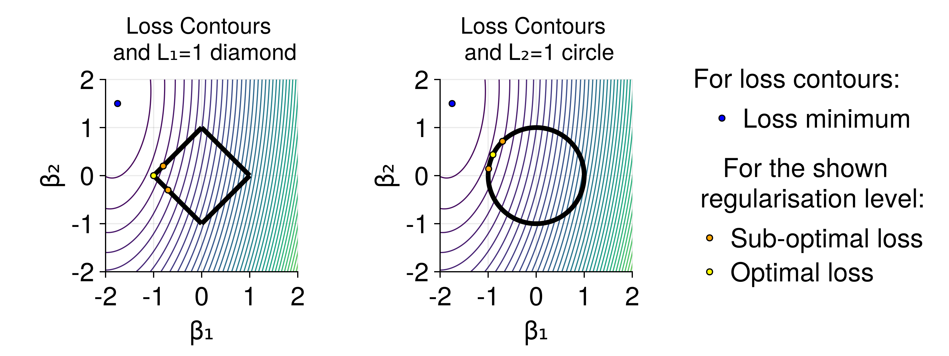
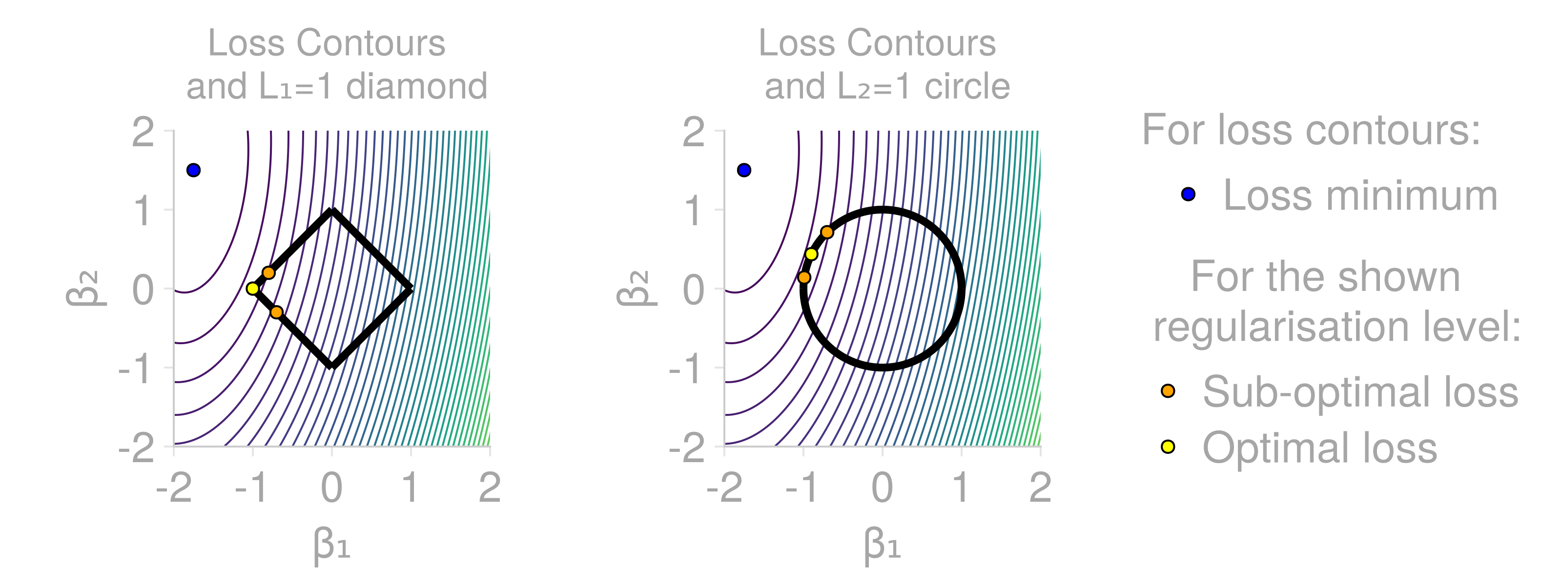
It is worth understanding the basic properties of L1 and L2 regularization and providing their alternative interpretations as probability distributions. The L1 and L2 penalties are defined as ${\mathcal{L}}_1=\lambda \times \sum _j|{\beta }_j|$ and ${\mathcal{L}}_2=\lambda \times \sum _j({\beta }_j{)}^2$ respectively, where $\lambda$ is a regularization constant (a hyper-parameter). Both penalties are meant to prevent overfitting to the training data but achieve this goal in different ways (see the plot below). Moreover, L1 regularization tends to result in sparser models, whereas L2 penalizes large parameter values much more heavily. For a more in-depth analysis and comparison of their properties, see "Regularization for Deep Learning" from "Deep Learning" by Goodfellow, Bengio, Courville.

The figure shows idealized loss surface contour lines (loss is equal on each line), the minimal loss value (blue dot) and shapes of ${\mathcal{L}}_1=1$ and ${\mathcal{L}}_2=1$ when $\lambda =1$. Note how, for the given level of regularization, due to the shapes of ${\mathcal{L}}_1$ (left plot) and ${\mathcal{L}}_2$ (right plot) different ${\beta }_1$ and ${\beta }_2$ values result in optimal loss (yellow dots). Namely, for ${\mathcal{L}}_1=1$ ${\beta }_2\approx 0$ is optimal, showcasing its sparsity-inducing property.

Due to their different properties, both L1 and L2 regularization have uses in different scenarios. Both L1 and L2 penalties can be linked to prior probability distributions of the neural network parameters. Specifically, L1 is proportional to $\text{Laplace}(0,\frac{1}{\lambda })$ and L2 is proportional to $\mathcal{N}(0,\frac{1}{\sqrt{2\lambda }})$ where $\lambda$ is the regularization constant.

Choosing Activation Functions

What activation functions are appropriate for the problems we typically deal with using DeepPumas? Our experience is that models are relatively robust to most architectural choices, but there are still a few things to consider.

Input/Hidden Layers

The MLPDomain default activation function is tanh as it is expressive and relatively computationally cheap. However, in situations where the inputs are not scaled, other functions may be better to avoid saturation, for example, elu or celu for which saturation is less of a problem, but they are not as expressive. Finally, it is worth mentioning that while relu is often great for many deep machine learning applications, it typically underperforms in small networks and with the fitting algorithms we tend to use in DeepPumas.

Output Layer

The activation function of the output layer warrants special attention because the wrong choice here may result in model instability, physically unrealistic model dynamics, or poor learning. As a rule of thumb, identity final layer is usually best, unless there are scientific reasons to restrict the output domain of a neural network. For example, if the expected outputs of a neural network should be in the interval $(0,1)$, then a sigmoid may be appropriate, whereas if the outputs should be positive but unbounded a softplus may be best. Note that even when using an unbounded activation function (e.g. identity or softplus), regularization applied to the output layer can still restrict the magnitude of the output. If this is undesirable then one can turn off output regularization (L1(λ, output=false)).

Choosing Neural Network Architecture

Similar to activation functions, there is usually a wide range of possible neural network architectures that perform similarly. Deeper and narrower neural networks tend to perform better than wider and shallower ones (for example, MLPDomain(3, 10, 10, 10, 1) as opposed to MLPDomain(3, 55, 1), both of which have a similar number of parameters). A rule of thumb when approximating small functions, like terms in a dynamical system, is to start with two hidden layers and to have slightly more nodes per hidden layer than we have inputs to the network. This allows the neural network to discover complex relationships between the inputs. In contrast, if the neural network contains fewer hidden units than inputs it compresses them/does dimensionality reduction and loses information before reaching the output layer.

Choosing Random Effect Inputs

Random effects enable models to appropriately account for systematic differences between individuals (or other entities being modeled) that could not be accounted for with the available data. Therefore, adding random effects as inputs to a neural network enables individualization of the average functional form that the network approximates. Every random effect provides one dimension along which we can account for individual differences.

Number of Random Effect Inputs in a Neural Network

Let us examine a well-established biological model – the Hill equation – as an example of selecting the number of random effects. The Hill equation is $\Theta (L)=\frac{[L{]}^n}{K_d+[L{]}^n}$ where $\Theta (L)$ is the fraction of receptors bound to some drug, $L$ is the drug concentration, $K_d$ is the dissociation constant and $n$ is the Hill coefficient. Assuming that both $K_d$ and $n$ vary between individuals, in order to get $NN(L)\approx \Theta (L)$ (a close approximation of the true function), we would need $NN(L,{\eta }_1,{\eta }_2)$ – a neural network with two random effects as inputs.

When using real data, contrary to the toy example above, we seldom know how many dimensions of variability are required to account for differences between individuals. This problem is not unique to DeepNLME models, as it is usually difficult to determine which parameters in classical NLME models need random effects for the model to fit well. However, this process is simpler for DeepNLME models since it is sufficient to guess how many random effects are needed and the neural network fitting determines the optimal way to use them. Furthermore, the flexibility of the neural networks to transform and utilize the random effects means that we can account for more outcome variability with fewer random effects. This is because classical NLME model parameters may have a covarying influence on the predicted individual outcomes. Similar to principal component analysis, where a large portion of data variability can often be covered by the first few principal components, a large portion of outcome variability can be accounted for by a few random effects when processed by a neural network.

Covariance Matrix Structure of Random Effects

Another practically relevant question is the structure of the covariance matrix $\mathrm{\Omega }$ of random effects. In definitions of the NLME models $\mathrm{\Omega }$ is often defined as diagonal and this decision stays practically sound when using random effects in neural networks. This is because the inclusion of off-diagonal elements in $\mathrm{\Omega }$ does not add much in terms of model expressiveness but makes the optimization significantly more difficult. Offloading the learning of relationships (if any) between the random effects inputs to the neural network is usually much simpler and a practically better idea due to its flexibility and modeling power. Moreover, having a diagonal $\mathrm{\Omega }$ incentivizes the discovery of an orthogonalized basis of outcome variability which makes it easier to use the sequential covariate modeling approach.

Using an Appropriate ODE Solver

ODE solvers can broadly be categorized into fixed (where $\mathrm{\Delta }t$ is fixed) and adaptive (where $\mathrm{\Delta }t$ is calculated to be as large as possible within the specified error bounds) time-step solvers. Some models display a phenomenon called stiffness – a feature of differential equation systems which, during its numerical solving, necessitates the usage of very small integration time steps due to rapid variation in its solution. Therefore, especially if a fixed time-step solver is used, numerical solving of stiff systems becomes very computationally expensive. Due to the prevalence and importance of stiff systems, there are ODE solvers that are specifically built to solve stiff systems efficiently (for a more in-depth discussion, see DifferentialEquations.jl documentation). Moreover, it is possible to algorithmically switch between stiff and non-stiff solvers, making use of the best features of either. By default, Pumas.jl uses an auto-switching (between Vern7 and Rodas5) ODE solver that should be a practically performant option in terms of speed and accuracy for a wide range of use cases. However, when dealing with very stiff systems it may be faster to use a stiff ODE solver. The ODE solver, along with other ODE solver arguments, e.g. error tolerances, can be specified in the fit function via the diffeq_options keyword argument:

fit(model,
    population,
    initial_parameters,
    algorithm,
    diffeq_options=(; alg=Rodas5P(), abstol=1e-16)
)

Setting ODE Solver Tolerances (ODE Solver, Inner and Outer Optimization)

ODE solver tolerances are an additional aspect to look into whenever the default settings do not produce desirable results. Inappropriate ODE tolerances are usually not difficult to troubleshoot due to warnings thrown by the ODE solver during optimization, for example

Interrupted. Larger maxiters is needed.

dt <= dtmin. Aborting. There is either an error in your model specification or the true solution is unstable.

NaN dt detected. Likely a NaN value in the state, parameters, or derivative value caused this outcome.

Instability detected. Aborting

Any of these may indicate errors in the model or that you are using a non-stiff ODE solver when a stiff one is warranted. However, it may also result from solver abstol or reltol values that are too large. Practically this means setting either abstol or reltol arguments in diffeq_options that are passed to the fit function. The values used in the default solver are abstol=1e-12 and reltol=1e-8 and due to floating point precision values smaller than 1e-16 should not be used. For a more in-depth discussion on ODE solver error tolerances see Numerical Error section in DifferentialEquations.jl documentation. Note that lower error tolerances will result in longer computation times because the solutions will be more accurate.

Optimization Options

In more advanced cases where desired results are not obtained a deeper dive into optimization options may be warranted. The backbone library for optimization is Optim.jl. There are many possible arguments and options that one may tweak in hopes of better performance (see Configurable Options). As a basic example, it is important to make sure that optimization terminates. This can be done in multiple ways. Optimization can be terminated by reaching tolerances for minimal change of the parameter vector (x_tol), optimization objective (f_tol) or gradient vector (g_tol). However, in a lot of instances, a more straightforward solution is to simply set the maximal number of iterations or a time_limit (in seconds) for the optimization run. This is done via the optim_options keyword argument of the fit function:

fit(model,
    population,
    initial_parameters,
    likelihood_approximation,
    optim_options=(; iterations = 10, 
        time_limit=3600, 
        x_tol=1e-3, 
        f_tol=1e-3, 
        g_tol=1e-3
    )
)

Delving deeper, some model optimization objectives (specifically marginal likelihood approximations LaplaceI, FOCE) are composed of the inner and the outer optimization loops. All other optimization objectives, such as FO, JointMAP or NaivePooled only have the outer loop. The inner loop finds the posterior mode of the random effect distribution which is then used in the outer loop to calculate the model parameter gradients with respect to the chosen marginal likelihood approximation. The default outer optimization algorithm is Optim.BFGS, which is a good option in a wide range of use cases. However, if the outer loop optimization algorithm customization is required (e.g. its line search algorithm or an alternative algorithm, e.g. Optim.LBFGS if memory is an issue), it can be done via the optim_alg keyword argument of the fit function:

fit(model,
    population,
    initial_parameters,
    likelihood_approximation,
    optim_options=(;iterations=100),
    optim_alg = Optim.LBFGS(linesearch=Optim.LineSearches.BackTracking())
)

It is also possible to customize the inner optimization loop (only applies to FOCE and LaplaceI), which uses NewtonTrustRegion as a default solver. The inner loop optimization algorithm should be specified as the first argument in the marginal likelihood approximation, whereas optimization options should be passed via Optim.Options as the second argument:

fit(
  model,
  population,
  initial_parameters,
  MAP(FOCE(;
    # Inner optimization options
    optim_alg = Optim.BFGS(linesearch=Optim.LineSearches.BackTracking()), 
    optim_options = (; iterations=10000),
  )), 
  # Outer optimization options
  optim_options=(; iterations = 10)
)

Note that if a fit fails, we recommend that you start by looking for issues with model misspecifications, neural network input/output scaling, the number of random effects used, or different likelihood approximations before tweaking the optimizers.